Reading in Previously Corrected Light Curves#
In this tutorial we will be reading in a light curve that we have already downloaded and corrected. If you have not done this, please see the plotting tutorial.
[1]:
import elk
import numpy as np

%config InlineBackend.figure_format = "retina" # Not required, only applicable for Jupyter Notebooks

# We will also need the two classes imported
from elk.ensemble import EnsembleLC
from elk.lightcurve import BasicLightcurve
[2]:
# define the path to your lightcurves
path = 'Corrected_LCs/'

# which Cluster would we like to read in
Name = "NGC 419"
[3]:
c = elk.ensemble.from_fits(path + Name + "output_table.fits")
From here, we have all of the available functions of a BasicLightcurve in elk!
Let’s look at the summary table.
[4]:
c.summary_table()
[4]:
Table length=1
| name | location | radius | log_age | has_data | n_obs | n_good_obs | which_sectors_good | n_failed_download | n_bad_quality | n_scatter_light | scattered_light_sectors | lc_lens |
|---|---|---|---|---|---|---|---|---|---|---|---|---|
| str7 | str18 | float64 | float64 | bool | int64 | int64 | str8 | int64 | int64 | int64 | str10 | str12 |
| NGC 419 | 23.58271, +61.1236 | 0.046 | 7.75 | True | 4 | 2 | [18, 24] | 0 | 0 | 2 | [[25, 58]] | [1103, 1224] |
Or we can plot one of the light curves
[5]:
c.lcs[0].plot()
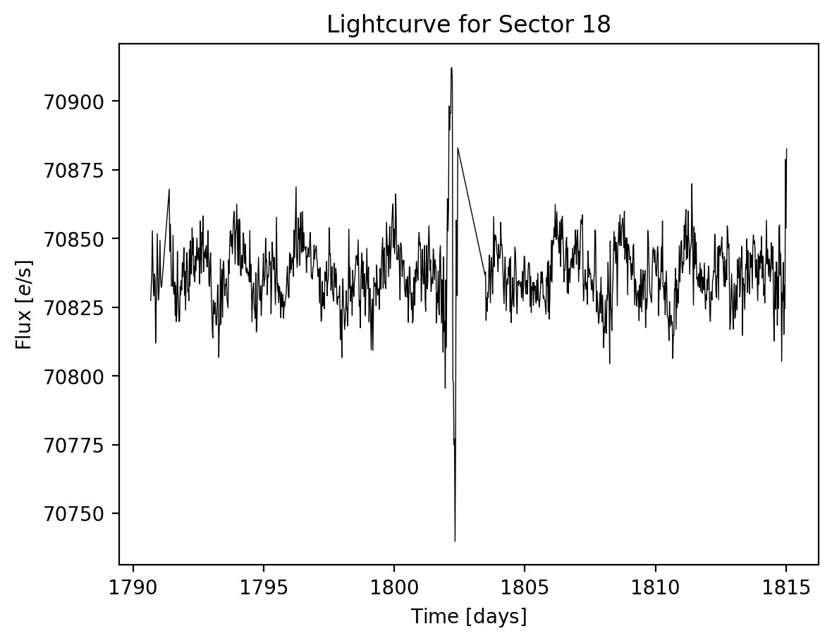
[5]:
(<Figure size 640x480 with 1 Axes>,
 <Axes: title={'center': 'Lightcurve for Sector 18'}, xlabel='Time $\\rm [days]$', ylabel='Flux $[e / {\\rm s}]$'>)
Note
This tutorial was generated from a Jupyter notebook that can be found here.