Lightcurve Analysis Plots

Intro

We can start by importing our favorite package: elk!

import elk
import numpy as np

%config InlineBackend.figure_format = "retina" # Not required, only applicable for Jupyter Notebooks

Lightcurve Setup

Now let’s do a simple ensemble lightcurve fit to NGC 419

c = elk.ensemble.EnsembleLC(output_path='.',
                            identifier='NGC 419',
                            location='23.58271, +61.1236',
                            radius=.046,
                            cluster_age=7.75,
                            cutout_size=25,
                            verbose=True,
                            minimize_memory=False)

c.create_output_table()

NGC 419 has 4 observations
Starting Quality Tests for Observation: 0

100%|█████████████████████████| 625/625 [00:24<00:00, 25.94it/s]

  Passed Quality Tests 
Starting Quality Tests for Observation: 1

100%|█████████████████████████| 625/625 [00:27<00:00, 22.42it/s]

  Passed Quality Tests 
Starting Quality Tests for Observation: 2

100%|█████████████████████████| 625/625 [00:24<00:00, 25.22it/s]

  Failed Scattered Light Test 
Starting Quality Tests for Observation: 3

100%|█████████████████████████| 625/625 [02:28<00:00,  4.20it/s]

  Failed Scattered Light Test 

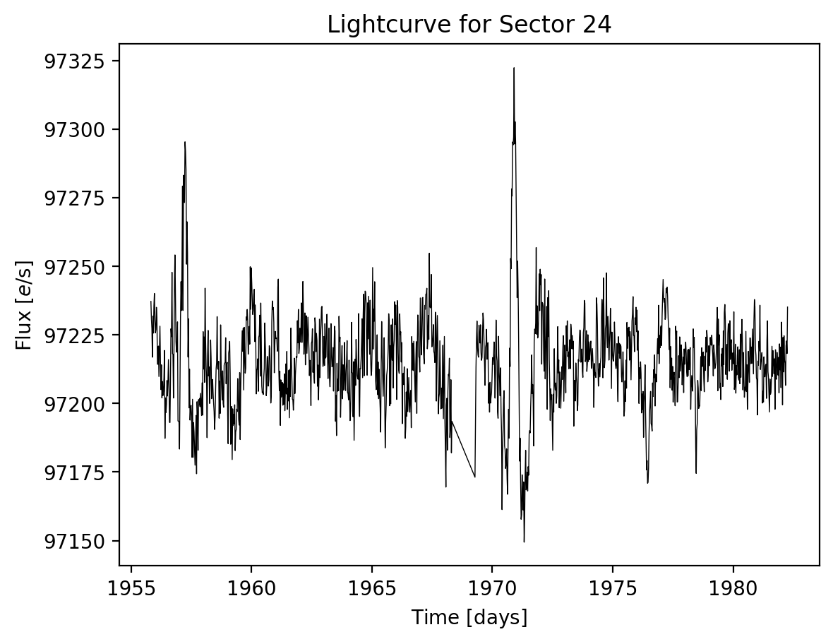
Plotting the lightcurve itself

Let’s quickly grab the 3rd lightcurve since that sector is usually looking lovely this time of year

lc = c.lcs[1]

The plotting of the lightcurve itself is rather straightforward!

lc.plot()

(<Figure size 640x480 with 1 Axes>,
 <Axes: title={'center': 'Lightcurve for Sector 24'}, xlabel='Time $\\rm [days]$', ylabel='Flux $[e / {\\rm s}]$'>)

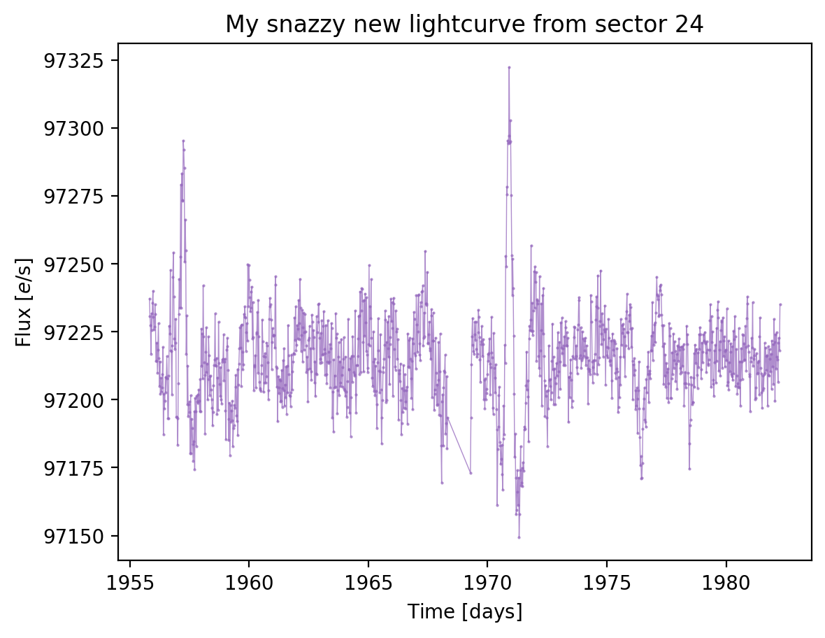
But it can also be very flexible if you like

lc.plot(title=f"My snazzy new lightcurve from sector {lc.sector}", color="tab:purple", marker="o", markersize=0.5, alpha=0.75)

(<Figure size 640x480 with 1 Axes>,
 <Axes: title={'center': 'My snazzy new lightcurve from sector 24'}, xlabel='Time $\\rm [days]$', ylabel='Flux $[e / {\\rm s}]$'>)

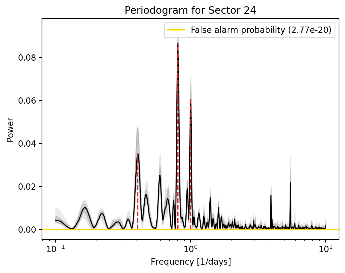
Periodogram plotting

Now let’s try plotting out the periodogram, for this we’ll need an array of frequencies

lc.to_periodogram(frequencies=np.logspace(-1, 1, 500), n_bootstrap=10)
_ = lc.plot_periodogram()

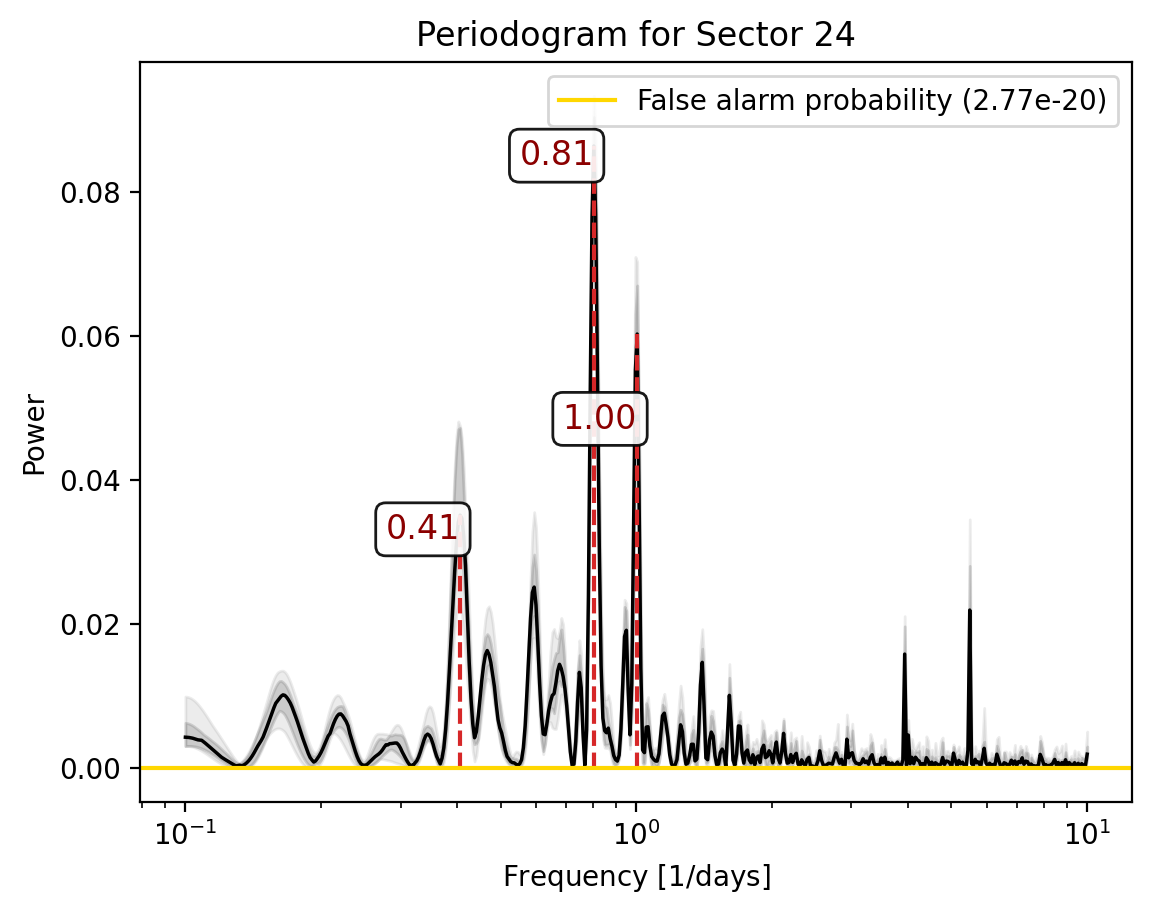
This plot can be similarly flexible in how you do things

fig, ax = lc.plot_periodogram(show=False)

for peak_ind in range(lc.stats["n_peaks"]):
    peak, peak_power = lc.stats["peak_freqs"][peak_ind], lc.stats["power_at_peaks"][peak_ind]
    ax.annotate(f'{peak:1.2f}', xy=(peak, peak_power), ha="right", va="bottom", color="darkred",
                fontsize="large", bbox=dict(boxstyle="round", fc="white", alpha=0.9))

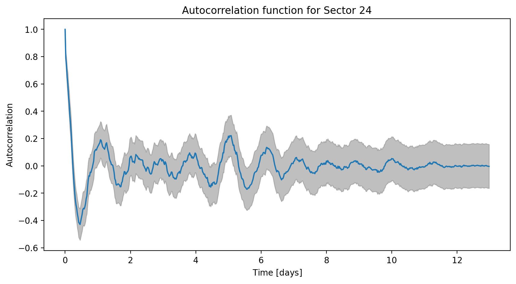
Plotting the autocorrelation function

The last of our trio of plots is the autocorrelation function. This one can be used in the same ways as above and can be called as

_ = lc.plot_acf()

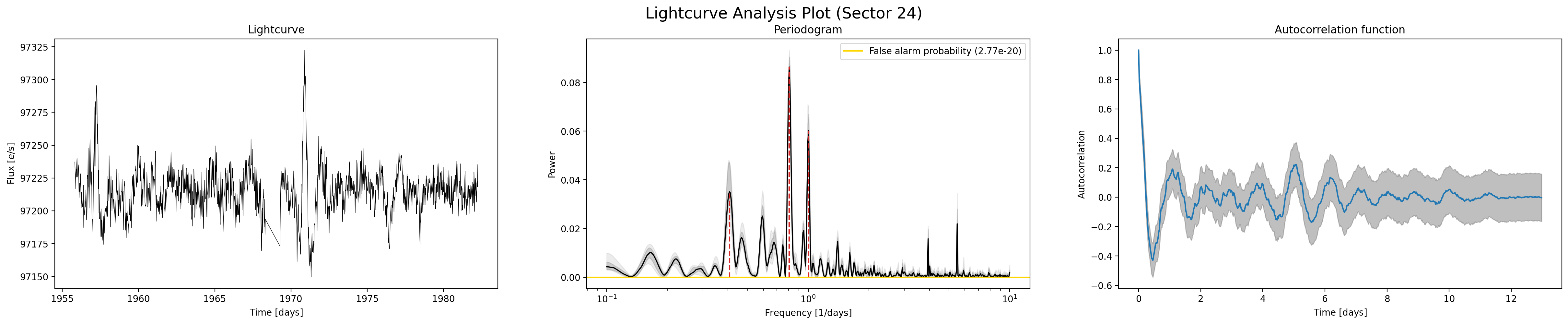
All together now

In many cases it can be convenient to get all of these plots quickly and for that purpose we have lc.analysis_plot()

_ = lc.analysis_plot()

Note

This tutorial was generated from a Jupyter notebook that can be found here.